






Visualize solutions#
The io module allows you to convert MutableTransition, Topology instances, and ProblemSets to Mermaid language with asmermaid(). The resulting diagrams can be embedded directly in Markdown. Initial and final states are rendered as rectangular nodes, intermediate states as rounded nodes, and compact interaction nodes as circles. Verbose solver-setting nodes remain rectangular. This is particularly useful after running find_solutions(), which produces a ReactionInfo object with a list of MutableTransition instances (see Generate transitions).
The same objects can also be converted to DOT language with asdot() and rendered with third-party libraries such as Graphviz. A few examples below demonstrate this alternative.
See also
The objects that the StateTransitionManager produces along the way, such as ProblemSets and QNResults, are rendered in Inspect intermediate results.
Topologies#
First of all, here is an example of how to visualize a group of Topology instances. We use create_isobar_topologies() and create_n_body_topology() to create a few standard topologies.
topology = create_n_body_topology(2, 4)
source = qrules.io.asmermaid(topology, markdown=True, render_initial_state_id=True)
Markdown(source)
        flowchart LR
    n_0["$$0$$"]
    n_1["$$1$$"]
    n_2["$$2$$"]
    n_3["$$3$$"]
    A["$$-1$$"]
    B["$$-2$$"]
    N0@{ shape: text, label: " " }
    B --- N0
    A --- N0
    N0 --- n_0
    N0 --- n_1
    N0 --- n_2
    N0 --- n_3
Note the IDs of the nodes is also rendered if there is more than node:
topologies = create_isobar_topologies(4)
Markdown(qrules.io.asmermaid(topologies, markdown=True))
        flowchart LR
    T0_0["$$0$$"]
    T0_1["$$1$$"]
    T0_2["$$2$$"]
    T0_3["$$3$$"]
    T0_A@{ shape: text, label: " " }
    T0_N0(("$$(0)$$"))
    T0_N1(("$$(1)$$"))
    T0_N2(("$$(2)$$"))
    T0_A --- T0_N0
    T0_N0 --- T0_N1
    T0_N0 --- T0_N2
    T0_N1 --- T0_0
    T0_N1 --- T0_1
    T0_N2 --- T0_2
    T0_N2 --- T0_3
    T1_0["$$0$$"]
    T1_1["$$1$$"]
    T1_2["$$2$$"]
    T1_3["$$3$$"]
    T1_A@{ shape: text, label: " " }
    T1_N0(("$$(0)$$"))
    T1_N1(("$$(1)$$"))
    T1_N2(("$$(2)$$"))
    T1_A --- T1_N0
    T1_N0 --- T1_N1
    T1_N0 --- T1_0
    T1_N1 --- T1_N2
    T1_N1 --- T1_1
    T1_N2 --- T1_2
    T1_N2 --- T1_3
This can be turned on or off with the arguments of asmermaid():
topologies = create_isobar_topologies(3)
Markdown(qrules.io.asmermaid(topologies, markdown=True, render_node=False))
        flowchart LR
    T0_0["$$0$$"]
    T0_1["$$1$$"]
    T0_2["$$2$$"]
    T0_A@{ shape: text, label: " " }
    T0_N0@{ shape: text, label: " " }
    T0_N1@{ shape: text, label: " " }
    T0_A --- T0_N0
    T0_N0 --- T0_N1
    T0_N0 --- T0_0
    T0_N1 --- T0_1
    T0_N1 --- T0_2
asmermaid() provides other options as well:
topologies = create_isobar_topologies(5)
some_topology = topologies[0]
source = qrules.io.asmermaid(
    some_topology,
    markdown=True,
    render_final_state_id=False,
    render_node=False,
    render_resonance_id=True,
)
Markdown(source)
        flowchart LR
    n_0@{ shape: text, label: " " }
    n_1@{ shape: text, label: " " }
    n_2@{ shape: text, label: " " }
    n_3@{ shape: text, label: " " }
    n_4@{ shape: text, label: " " }
    A@{ shape: text, label: " " }
    N0@{ shape: text, label: " " }
    N1@{ shape: text, label: " " }
    N2@{ shape: text, label: " " }
    N3@{ shape: text, label: " " }
    n_5("$$5$$")
    n_6("$$6$$")
    n_7("$$7$$")
    A --- N0
    N0 --- n_5
    n_5 --- N1
    N0 --- n_0
    N1 --- n_6
    n_6 --- N2
    N1 --- n_1
    N2 --- n_7
    n_7 --- N3
    N2 --- n_2
    N3 --- n_3
    N3 --- n_4
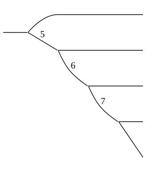
The same options are available for asdot(); its output can be rendered with graphviz.Source:
dot = qrules.io.asdot(
    some_topology,
    render_final_state_id=False,
    render_node=False,
    render_resonance_id=True,
)
graphviz.Source(dot)
StateTransitions#
After finding the Quantum number solutions, QRules finds Particle definitions that match these quantum numbers. All these steps are hidden in the convenience functions StateTransitionManager.find_solutions() and generate_transitions(). In the following, we’ll visualize the allowed transitions for the decay \(\psi' \to \gamma\eta\eta\) as an example.
import qrules

reaction = qrules.generate_transitions(
    initial_state="psi(2S)",
    final_state=["gamma", "eta", "eta"],
    allowed_interaction_types="EM",
)
As noted in 3. Find solutions, the transitions contain all spin projection combinations (which is necessary for the ampform package). It is possible to convert all these solutions to Mermaid language with asmermaid(). To avoid visualizing all solutions, we just take a subset of the transitions:
some_transitions = reaction.transitions[::50][:3]
source = qrules.io.asmermaid(some_transitions)
This str of Mermaid language for the list of MutableTransition instances can be wrapped in a Mermaid code fence with markdown=True and displayed directly as Markdown:
source = qrules.io.asmermaid(some_transitions, markdown=True, render_node=False)
Markdown(source)
        flowchart LR
    T0_0["$$0: \gamma\left[\text{-}1\right]$$"]
    T0_1["$$1: \eta\left[0\right]$$"]
    T0_2["$$2: \eta\left[0\right]$$"]
    T0_N0["$$\psi(2S)\left[\text{-}1\right]$$"]
    T0_N1@{ shape: text, label: " " }
    T0_3("$$f_{2}(2340)\left[\text{-}2\right]$$")
    T0_N0 --- T0_3
    T0_3 --- T0_N1
    T0_N0 --- T0_0
    T0_N1 --- T0_1
    T0_N1 --- T0_2
    T1_0["$$0: \gamma\left[\text{-}1\right]$$"]
    T1_1["$$1: \eta\left[0\right]$$"]
    T1_2["$$2: \eta\left[0\right]$$"]
    T1_N0["$$\psi(2S)\left[\text{-}1\right]$$"]
    T1_N1@{ shape: text, label: " " }
    T1_3("$$f_{2}^\prime(1525)\left[0\right]$$")
    T1_N0 --- T1_3
    T1_3 --- T1_N1
    T1_N0 --- T1_0
    T1_N1 --- T1_1
    T1_N1 --- T1_2
    T2_0["$$0: \gamma\left[\text{-}1\right]$$"]
    T2_1["$$1: \eta\left[0\right]$$"]
    T2_2["$$2: \eta\left[0\right]$$"]
    T2_N0["$$\psi(2S)\left[\text{-}1\right]$$"]
    T2_N1@{ shape: text, label: " " }
    T2_3("$$a_{0}(980)^{0}\left[0\right]$$")
    T2_N0 --- T2_3
    T2_3 --- T2_N1
    T2_N0 --- T2_0
    T2_N1 --- T2_1
    T2_N1 --- T2_2
You can also serialize the Mermaid source to a file with io.write(). The file extension for a Mermaid file is .mmd:
qrules.io.write(reaction, "decay_topologies_with_spin.mmd")
Alternatively, io.write() can serialize the same object as DOT when the .gv file extension is used:
qrules.io.write(reaction, "decay_topologies_with_spin.gv")
Collapse graphs#
Since this list of all possible spin projections transitions is rather long, it is often useful to use strip_spin=True or collapse_graphs=True to bundle comparable graphs. First, strip_spin=True allows one collapse (ignore) the spin projections (we again show a selection only):
first_transitions = reaction.transitions[:3]
source = qrules.io.asmermaid(first_transitions, markdown=True, strip_spin=True)
Markdown(source)
        flowchart LR
    T0_0["$$0: \gamma$$"]
    T0_1["$$1: \eta$$"]
    T0_2["$$2: \eta$$"]
    T0_N0["$$\psi(2S)$$"]
    T0_N1@{ shape: text, label: " " }
    T0_3("$$a_{2}(1320)^{0}$$")
    T0_N0 --- T0_3
    T0_3 --- T0_N1
    T0_N0 --- T0_0
    T0_N1 --- T0_1
    T0_N1 --- T0_2
    T1_0["$$0: \gamma$$"]
    T1_1["$$1: \eta$$"]
    T1_2["$$2: \eta$$"]
    T1_N0["$$\psi(2S)$$"]
    T1_N1@{ shape: text, label: " " }
    T1_3("$$a_{0}(980)^{0}$$")
    T1_N0 --- T1_3
    T1_3 --- T1_N1
    T1_N0 --- T1_0
    T1_N1 --- T1_1
    T1_N1 --- T1_2
or, with stripped node properties:
source = qrules.io.asmermaid(
    first_transitions,
    markdown=True,
    render_node=True,
    strip_spin=True,
)
Markdown(source)
        flowchart LR
    T0_0["$$0: \gamma$$"]
    T0_1["$$1: \eta$$"]
    T0_2["$$2: \eta$$"]
    T0_A["$$\psi(2S)$$"]
    T0_N0(("$$\begin{gathered} L = 0 \\\ S = 1 \\\ P = \text{+}1 \end{gathered}$$"))
    T0_N1(("$$\begin{gathered} L = 2 \\\ S = 0 \\\ P = \text{+}1 \end{gathered}$$"))
    T0_3("$$a_{2}(1320)^{0}$$")
    T0_A --- T0_N0
    T0_N0 --- T0_3
    T0_3 --- T0_N1
    T0_N0 --- T0_0
    T0_N1 --- T0_1
    T0_N1 --- T0_2
    T1_0["$$0: \gamma$$"]
    T1_1["$$1: \eta$$"]
    T1_2["$$2: \eta$$"]
    T1_A["$$\psi(2S)$$"]
    T1_N0(("$$\begin{gathered} L = 2 \\\ S = 1 \\\ P = \text{+}1 \end{gathered}$$"))
    T1_N1(("$$\begin{gathered} L = 0 \\\ S = 0 \\\ P = \text{+}1 \end{gathered}$$"))
    T1_3("$$a_{0}(980)^{0}$$")
    T1_A --- T1_N0
    T1_N0 --- T1_3
    T1_3 --- T1_N1
    T1_N0 --- T1_0
    T1_N1 --- T1_1
    T1_N1 --- T1_2
    T2_0["$$0: \gamma$$"]
    T2_1["$$1: \eta$$"]
    T2_2["$$2: \eta$$"]
    T2_A["$$\psi(2S)$$"]
    T2_N0(("$$\begin{gathered} L = 0 \\\ S = 1 \\\ P = \text{+}1 \end{gathered}$$"))
    T2_N1(("$$\begin{gathered} L = 0 \\\ S = 0 \\\ P = \text{+}1 \end{gathered}$$"))
    T2_3("$$a_{0}(980)^{0}$$")
    T2_A --- T2_N0
    T2_N0 --- T2_3
    T2_3 --- T2_N1
    T2_N0 --- T2_0
    T2_N1 --- T2_1
    T2_N1 --- T2_2
Note
By default, asmermaid() renders edge IDs, because they represent the (final) state IDs as well. This can be disabled with render_final_state_id=False.
If that list is still too much, there is collapse_graphs=True, which bundles all graphs with the same final state groupings:
source = qrules.io.asmermaid(
    reaction, collapse_graphs=True, markdown=True, render_node=False
)
Markdown(source)
        flowchart LR
    T0_0["$$0: \gamma$$"]
    T0_1["$$1: \eta$$"]
    T0_2["$$2: \eta$$"]
    T0_N0["$$\psi(2S)$$"]
    T0_N1@{ shape: text, label: " " }
    T0_3("$$\begin{array}{ll} b_{1}(1235)^{0} & \omega(1650) \\\ h_{1}(1170) & \phi(1020) \\\ h_{1}(1415) & \phi(1680) \\\ J/\psi(1S) & \rho(770)^{0} \\\ \omega(782) & \rho(1450)^{0} \\\ \omega(1420) & \rho(1700)^{0} \end{array}$$")
    T0_N0 --- T0_3
    T0_3 --- T0_N1
    T0_N0 --- T0_1
    T0_N1 --- T0_0
    T0_N1 --- T0_2
    T1_0["$$0: \gamma$$"]
    T1_1["$$1: \eta$$"]
    T1_2["$$2: \eta$$"]
    T1_N0["$$\psi(2S)$$"]
    T1_N1@{ shape: text, label: " " }
    T1_3("$$\begin{array}{llll} a_{0}(980)^{0} & \chi_{c2}(1P) & f_{2}^\prime(1525) & f_{0}(2020) \\\ a_{2}(1320)^{0} & f_{0}(500) & f_{0}(1500) & f_{2}(2010) \\\ a_{0}(1450)^{0} & f_{0}(980) & f_{2}(1565) & f_{2}(2150) \\\ a_{2}(1700)^{0} & f_{2}(1270) & f_{0}(1710) & f_{2}(2300) \\\ \chi_{c0}(1P) & f_{0}(1370) & f_{2}(1950) & f_{2}(2340) \end{array}$$")
    T1_N0 --- T1_3
    T1_3 --- T1_N1
    T1_N0 --- T1_0
    T1_N1 --- T1_1
    T1_N1 --- T1_2
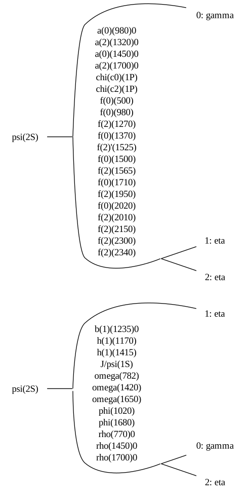
The same options also work with asdot(), for example:
dot = qrules.io.asdot(reaction, collapse_graphs=True, render_node=False)
graphviz.Source(dot)
Other state renderings#
The convert() method makes it possible to convert the types of its states. This for instance allows us to only render the spin states on in a Transition:
spin_transitions = sorted({
    t.convert(lambda s: Spin(s.particle.spin, s.spin_projection))
    for t in reaction.transitions
})
some_spin_transitions = spin_transitions[::67][:3]
source = qrules.io.asmermaid(some_spin_transitions, markdown=True, render_node=True)
Markdown(source)
        flowchart LR
    T0_0["$$0: \left|1,\text{+}1\right\rangle$$"]
    T0_1["$$1: \left|0,0\right\rangle$$"]
    T0_2["$$2: \left|0,0\right\rangle$$"]
    T0_A["$$\left|1,\text{+}1\right\rangle$$"]
    T0_N0(("$$\begin{gathered} L = \left|2,0\right\rangle \\\ S = \left|1,\text{+}1\right\rangle \\\ P = \text{+}1 \end{gathered}$$"))
    T0_N1(("$$\begin{gathered} L = \left|2,0\right\rangle \\\ S = \left|1,\text{+}1\right\rangle \\\ P = \text{+}1 \end{gathered}$$"))
    T0_3("$$\left|1,\text{-}1\right\rangle$$")
    T0_A --- T0_N0
    T0_N0 --- T0_3
    T0_3 --- T0_N1
    T0_N0 --- T0_1
    T0_N1 --- T0_0
    T0_N1 --- T0_2
    T1_0["$$0: \left|1,\text{-}1\right\rangle$$"]
    T1_1["$$1: \left|0,0\right\rangle$$"]
    T1_2["$$2: \left|0,0\right\rangle$$"]
    T1_A["$$\left|1,\text{-}1\right\rangle$$"]
    T1_N0(("$$\begin{gathered} L = \left|2,0\right\rangle \\\ S = \left|1,0\right\rangle \\\ P = \text{+}1 \end{gathered}$$"))
    T1_N1(("$$\begin{gathered} L = \left|0,0\right\rangle \\\ S = \left|1,\text{-}1\right\rangle \\\ P = \text{+}1 \end{gathered}$$"))
    T1_3("$$\left|1,0\right\rangle$$")
    T1_A --- T1_N0
    T1_N0 --- T1_3
    T1_3 --- T1_N1
    T1_N0 --- T1_1
    T1_N1 --- T1_0
    T1_N1 --- T1_2
    T2_0["$$0: \left|1,\text{-}1\right\rangle$$"]
    T2_1["$$1: \left|0,0\right\rangle$$"]
    T2_2["$$2: \left|0,0\right\rangle$$"]
    T2_A["$$\left|1,\text{-}1\right\rangle$$"]
    T2_N0(("$$\begin{gathered} L = \left|0,0\right\rangle \\\ S = \left|1,\text{-}1\right\rangle \\\ P = \text{+}1 \end{gathered}$$"))
    T2_N1(("$$\begin{gathered} L = \left|0,0\right\rangle \\\ S = \left|0,0\right\rangle \\\ P = \text{+}1 \end{gathered}$$"))
    T2_3("$$\left|0,0\right\rangle$$")
    T2_A --- T2_N0
    T2_N0 --- T2_3
    T2_3 --- T2_N1
    T2_N0 --- T2_0
    T2_N1 --- T2_1
    T2_N1 --- T2_2
Or any other properties of a State, such as masses or \(J^{PC}(I^G)\) numbers:
        flowchart LR
    T0_0["$$0: 0.0$$"]
    T0_1["$$1: 0.548$$"]
    T0_2["$$2: 0.548$$"]
    T0_N0["$$3.686$$"]
    T0_N1@{ shape: text, label: " " }
    T0_3("$$1.72±0.25$$")
    T0_N0 --- T0_3
    T0_3 --- T0_N1
    T0_N0 --- T0_1
    T0_N1 --- T0_0
    T0_N1 --- T0_2
    T1_0["$$0: 0.0$$"]
    T1_1["$$1: 0.548$$"]
    T1_2["$$2: 0.548$$"]
    T1_N0["$$3.686$$"]
    T1_N1@{ shape: text, label: " " }
    T1_3("$$0.775±0.147$$")
    T1_N0 --- T1_3
    T1_3 --- T1_N1
    T1_N0 --- T1_1
    T1_N1 --- T1_0
    T1_N1 --- T1_2
    T2_0["$$0: 0.0$$"]
    T2_1["$$1: 0.548$$"]
    T2_2["$$2: 0.548$$"]
    T2_N0["$$3.686$$"]
    T2_N1@{ shape: text, label: " " }
    T2_3("$$1.706±0.38$$")
    T2_N0 --- T2_3
    T2_3 --- T2_N1
    T2_N0 --- T2_0
    T2_N1 --- T2_1
    T2_N1 --- T2_2
    T3_0["$$0: 0.0$$"]
    T3_1["$$1: 0.548$$"]
    T3_2["$$2: 0.548$$"]
    T3_N0["$$3.686$$"]
    T3_N1@{ shape: text, label: " " }
    T3_3("$$0.6±0.45$$")
    T3_N0 --- T3_3
    T3_3 --- T3_N1
    T3_N0 --- T3_0
    T3_N1 --- T3_1
    T3_N1 --- T3_2
        flowchart LR
    T0_0["$$0: 1^{--}$$"]
    T0_1["$$1: 0^{-+}\left(0^{+}\right)$$"]
    T0_2["$$2: 0^{-+}\left(0^{+}\right)$$"]
    T0_N0["$$1^{--}\left(0^{-}\right)$$"]
    T0_N1@{ shape: text, label: " " }
    T0_3("$$\begin{gathered} 1^{+-}\left(0^{-}\right) \\\ 1^{+-}\left(1^{+}\right) \\\ 1^{--}\left(0^{-}\right) \\\ 1^{--}\left(1^{+}\right) \end{gathered}$$")
    T0_N0 --- T0_3
    T0_3 --- T0_N1
    T0_N0 --- T0_1
    T0_N1 --- T0_0
    T0_N1 --- T0_2
    T1_0["$$0: 1^{--}$$"]
    T1_1["$$1: 0^{-+}\left(0^{+}\right)$$"]
    T1_2["$$2: 0^{-+}\left(0^{+}\right)$$"]
    T1_N0["$$1^{--}\left(0^{-}\right)$$"]
    T1_N1@{ shape: text, label: " " }
    T1_3("$$\begin{gathered} 0^{++}\left(0^{+}\right) \\\ 0^{++}\left(1^{-}\right) \\\ 2^{++}\left(0^{+}\right) \\\ 2^{++}\left(1^{-}\right) \end{gathered}$$")
    T1_N0 --- T1_3
    T1_3 --- T1_N1
    T1_N0 --- T1_0
    T1_N1 --- T1_1
    T1_N1 --- T1_2
Tip
Note that collapsing the graphs also works for custom edge properties.
Styling#
asmermaid() accepts styling arguments for the diagram, its edges, and its nodes through figure_style, edge_style, and node_style, respectively:
some_transition = reaction.transitions[0]
source = qrules.io.asmermaid(
    some_transition,
    edge_style={
        "color": "red",
        "fontcolor": "blue",
        "fontsize": 25,
    },
    figure_style={"bgcolor": "white"},
    markdown=True,
    node_style={
        "color": "gray",
        "fill": "lightgray",
        "stroke": "black",
    },
    render_node=True,
)
Markdown(source)
        flowchart LR
classDef default fill:white
    n_0["$$\textcolor{gray}{0: \gamma\left[\text{-}1\right]}$$"]
    n_1["$$\textcolor{gray}{1: \eta\left[0\right]}$$"]
    n_2["$$\textcolor{gray}{2: \eta\left[0\right]}$$"]
    A["$$\textcolor{gray}{\psi(2S)\left[\text{-}1\right]}$$"]
    N0(("$$\textcolor{gray}{\begin{gathered} L = \left|0,0\right\rangle \\\ S = \left|1,\text{-}1\right\rangle \\\ P = \text{+}1 \end{gathered}}$$"))
    N1(("$$\textcolor{gray}{\begin{gathered} L = \left|0,0\right\rangle \\\ S = \left|0,0\right\rangle \\\ P = \text{+}1 \end{gathered}}$$"))
    n_3("$$\textcolor{blue}{a_{0}(980)^{0}\left[0\right]}$$")
    A --- N0
    N0 --- n_3
    n_3 --- N1
    N0 --- n_0
    N1 --- n_1
    N1 --- n_2
    style n_0 color:gray,fill:lightgray,stroke:black
    style n_1 color:gray,fill:lightgray,stroke:black
    style n_2 color:gray,fill:lightgray,stroke:black
    style A color:gray,fill:lightgray,stroke:black
    style N0 color:gray,fill:lightgray,stroke:black
    style N1 color:gray,fill:lightgray,stroke:black
    style n_3 stroke:red,color:blue,font-size:25px
    linkStyle 0 stroke:red,color:blue,font-size:25px
    linkStyle 1 stroke:red,color:blue,font-size:25px
    linkStyle 2 stroke:red,color:blue,font-size:25px
    linkStyle 3 stroke:red,color:blue,font-size:25px
    linkStyle 4 stroke:red,color:blue,font-size:25px
    linkStyle 5 stroke:red,color:blue,font-size:25px
For DOT output, asdot() takes Graphviz attributes. Examples are size, color, and fontcolor. Edges and nodes can be styled with edge_style and node_style, respectively:
dot = qrules.io.asdot(
    some_transition,
    bgcolor="white",
    edge_style={
        "arrowhead": "open",
        "color": "red",
        "fontcolor": "blue",
        "fontsize": 25,
    },
    node_style={
        "color": "gray",
        "penwidth": 2,
        "shape": "ellipse",
        "style": "dashed",
    },
    render_node=True,
    size=12,
)
graphviz.Source(dot)

By default, Mermaid renders labels with LaTeX. This can be disabled with the latex argument of asmermaid():
source = qrules.io.asmermaid(
    some_transition,
    latex=False,
    markdown=True,
    render_node=True,
)
Markdown(source)
        flowchart LR
    n_0["0: gamma[-1]"]
    n_1["1: eta[0]"]
    n_2["2: eta[0]"]
    A["psi(2S)[-1]"]
    N0(("L=|0,0⟩<br/>S=|1,-1⟩<br/>P=+1"))
    N1(("L=|0,0⟩<br/>S=|0,0⟩<br/>P=+1"))
    n_3("a(0)(980)0[0]")
    A --- N0
    N0 --- n_3
    n_3 --- N1
    N0 --- n_0
    N1 --- n_1
    N1 --- n_2